¶ Keys to Understanding
KEY CONCEPT: In Inferential Statistics, p is the Probability of an Alpha Error ("False Positive")
In Inferential Statistics, we use information from a smaller group (sample) to estimate a characteristic (like the average, i.e Mean) of the larger group or process it came from.
Because this is just an estimate, there's a chance we might make a mistake. One common mistake is called the Alpha Error, also known as "Type I Error" or "False Positive."
The Alpha Error occurs when we mistakenly think there is a significant difference or change, but in reality, there is not.
For instance, we might wrongly believe there's a big gap in average values between two groups, assume a process has changed when it hasn't, or incorrectly think a medical treatment is effective when it's not.
In Hypothesis Testing, there's something called the Null Hypothesis, which suggests there's no difference or change. Making the mistake of rejecting this idea when it's actually true can lead to different situations.
We use the symbol p to represent the probability of encountering an Alpha Error, a "False Positive". This probability is calculated when we're doing Inferential Statistical analysis, like in a t-test or ANOVA.
Alpha Errors happen when our small sample doesn't really represent the entire group or process it came from. If our sample is big enough, most of them will give a good idea of what the whole group is like, but some might not. The value of p helps us understand how likely it is that our sample is not a good representation and might lead to an Alpha Error.
KEY CONCEPT: Alpha is the highest value of p that we are willing to tolerate and still say that a difference, change, or effect observed in the Sample is "Statistically Significant".
"Alpha" is a term used in statistics to describe a specific kind of mistake called the Alpha Error. When we talk about "Alpha" as a noun, we're referring to a value denoted by p that sets the boundary for acceptable probabilities.
For example, if we're okay with a 5% chance of making a False Positive error, we choose 𝛼 (Alpha) as 5%. This means we tolerate p values less than or equal to 5%, but not greater than 5%.
It's crucial to decide on Alpha before collecting sample data to maintain the credibility of our test or experiment. If we look at the data first, it might influence our choice of Alpha.
Instead of directly starting with Alpha, it's often more natural to think about a Level of Confidence first. Subtracting this from 100% gives us Alpha.
For instance:
If we want to be 95% confident, we go for a 95% Level of Confidence.
By definition, 𝜶 = 100% – Confidence Level = 5% (and, so Confidence Level = 100% – 𝛼).

Alpha is also known as the "Level of Significance" or "Significance Level".
- If
pis less than or equal to 𝜶, the observed difference, change, or effect in our sample data is considered "Statistically Significant". - If
pis greater than 𝜶, it's not deemed statistically significant.
Common choices for Alpha include 10% (0.1), 5% (0.05), 1% (0.01), 0.5% (0.005), and 0.1% (0.001).
But why not always choose the lowest Alpha possible? Well, it's a tradeoff between Alpha (Type I) Error and Beta (Type II) Error, or in simpler terms, between a False Positive and a False Negative. Lowering the chance of one increases the chance of the other.

Choosing 𝜶 = 0.05 (5%) is generally seen as a balanced and accepted choice for most applications.
KEY CONCEPT: Alpha is a Cumulative Probability, represented as an areaunder the curve, at one or both tails of a Probability Distribution. p is also a Cumulative Probability.
Displayed below are illustrations of the Standard Normal Distribution. The horizontal axis represents the Test Statistic, denoted as z. Each point on the curve corresponds to the Probability of the z value directly beneath it.
In statistics, the Probabilities of individual points are typically less informative than the Probabilities associated with ranges of values. These cumulative probabilities are referred to as Cumulative Probabilities. The Cumulative Probability for a specific range is determined by calculating the area under the curve above that range. The Cumulative Probability for all values under the curve equals 100%.
The initial step involves choosing a value for Alpha, commonly set at 5%. This value guides the size of the shaded area beneath the curve. Depending on the nature of the problem being addressed, we position the shaded area (𝜶) beneath the left tail, the right tail, or both tails.

If the analysis involves only one tail, it is referred to as "1-tailed" or "1-sided" (alternatively "left-tailed" or "right-tailed"), and the Alpha value is entirely allocated to that specific side of the curve.
On the other hand, if the analysis involves both tails, it is termed a "2-tailed" or "2-sided" analysis. In such instances, the Alpha value is divided by two, with half assigned to each tail of the curve.
KEY CONCEPT: In Hypothesis Testing, if p ≤ 𝜶, Reject the Null Hypothesis. If p > 𝜶, Accept (Fail to Reject) the Null Hypothesis.
In Hypothesis testing, p is compared to 𝜶 (Alpha), in order to determine what we can conclude from the test.
Hypothesis Testing starts with a Null Hypothesis – a statement that there is no (Statistically Significant) difference, change, or effect.
We select a value for Alpha (say 5%) and then collect a Sample of data. Next, a statistical test (like a t-test or F-test) is performed. The test output includes a value for p, also called p-value.
p is the Probability of an Alpha Error, a False Positive, that is, the Probability that any difference, effect, or change shown by the Sample data is not Statistically Significant.
If p is small enough, then we can be confident that there really is a difference, change, or effect.
How small is small enough? Less than or equal to Alpha.
Remember, we picked Alpha as the upper boundary for the values of p which indicate a tolerable Probability of an Alpha Error.
So, p > 𝛼 is an unacceptably high Probability of an Alpha Error.
How confident can we be? As confident as the Level of Confidence.
For example, with a 5% Alpha (Significance Level), we have a 100% – 5% = 95% Confidence Level.
So, ...
If p ≤ 𝜶, then we conclude that:
- the Probability of an Alpha Error is within the range we said we would tolerate, so the observed difference, change, or effect we are testing is "Statistically Significant".
- in a Hypothesis test, we would Reject the Null Hypothesis.
- the smaller the p-value, the stronger the evidence for this conclusion.
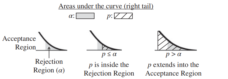
Let's look at the graph below, this is for a 1-tailed test (right-tailed), in which the shaded area represents 𝜶 (Alpha) and the hatched areas represent p.
- Left graph below: in Hypothesis Testing, some use the term "Acceptance Region" or "Non-critical Region" for the unshaded white area under the Distribution curve, and "Rejection Region" or "Critical Region" for the shaded area representing Alpha.

- Center graph: if the hatched area representing p is entirely in the shaded Rejection Region (because p ≤ 𝜶) we Reject the Null Hypothesis.
- Right graph: If p extends into the white Acceptance Region (because p > 𝜶), we Accept (or "Fail to Reject") the Null Hypothesis.
KEY CONCEPT: Alpha defines the Critical Value(s) of Test Statistics, such as z, t, F, or Chi-Square. The Critical Value or Values, in turn, define the Confidence Interval.
We explained how Alpha plays a key role in the Hypothesis Testing method of Inferential Statistics. It is also an integral part of the other main method - Confidence Intervals.
For example:
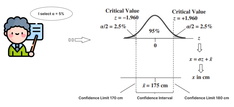
Let’s say we want a Confidence Interval around the Mean height of males. It is also illustrated in the following concept flow diagram (follow the arrows):

Top part of the diagram:
- The person performing the analysis selects a value for Alpha.
- Alpha – split into two halves – is shown as the shaded areas under the two tails of the curve of a Test Statistic, like z.
- Tables or calculations provide the values of the Test Statistic which form the boundaries of these shaded 𝛼/2 areas. In this example, z = −1.960 and z = +1.960.
- These values are the Critical Values of the Test Statistic for 𝛼 = 5%. They are in the units of the Test Statistic (z is in units of Standard Deviations).
Bottom part of the diagram:
- A Sample of data is collected and a Statistic (e.g., the Sample Mean, x) is calculated (175 cm in this example).
- To make use of the Critical Values in the real world, we need to convert the Test Statistic Values into real-world values – like centimeters in the example above.
There are different conversion formulas for different Test Statistics and different tests. In this illustration, z is the Test Statistic and it is defined as z = (x − x)/𝜎. So x = 𝜎z + x. We multiply 𝜎 by each critical value of z (−1.960 and +1.960), and we add those to the Sample Mean (175 cm).
- That converts the Critical Values −1.960 and +1.960 into the Confidence Limits of 170 and 180 cm.
- These Confidence Limits define the lower and upper boundaries of the Confidence Interval.
¶ Conclusion
In summary, Inferential Statistics employs sample data to estimate larger group characteristics, introducing potential errors like the Alpha Error. Alpha, denoted as 𝛼, signifies the permissible probability for an Alpha Error. Choosing 𝛼 involves balancing Type I and Type II errors, impacting confidence levels and significance. The interaction between Alpha and p-values guides decisions in Hypothesis Testing, influencing Null Hypothesis acceptance or rejection. Alpha's role extends to defining critical values in Test Statistics, shaping Confidence Intervals for comprehensive statistical inferences.
References:
[1] Statistics from A to Z - Confusing Concepts Clarified (ANDREW A. JAWLIK)